The LTER–Sweet Cherry Model v1 is a web-based decision-support tool that uses daily temperature and solar radiation data to generate seasonal estimates of floral dormancy progression (LTER), floral relative water content (RWC), and cold hardiness (LT, LT10 and LT50) for 12 cultivars and at the species level. The application provides interactive time-series visualizations designed to help growers, researchers and industry professionals interpret both seasonal bud status and potential frost risk.
Model outputs
Model development used physiological datasets collected over multiple seasons in Prosser, Washington (2019–2022), including dormancy status, water relations and cold hardiness measurements aligned with daily atmospheric inputs (Magby 2025). Integration with WSU AgWeatherNet is expected in the near future. The current version is available at this link.
Dormancy progression (LTER). Low Temperature Exotherm Ratios (LTER) are a physiological index derived from differential thermal analysis research that reflects seasonal changes in bud dormancy status (Magby et al. 2022). Values range from 0 to 1 and reflect seasonal transitions toward spring development (Figure 1).
The LTER panel shows seasonal trajectories with reference threshold lines and developmental stage windows [Green Side (l-green), Green Tip (d-green), Tight Cluster (yellow), Popcorn (orange) and Bloom (red)] to facilitate seasonal interpretation. Line chart of predicted LTER (y-axis) versus date (x-axis).
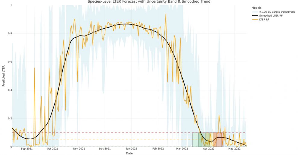 Figure 1. Example of seasonal LTER trajectory for Yakima, Washington (2021–2022), generated using the random forest (RF) model.
Relative water content (RWC). Relative water content (RWC) reflects the hydration status of floral buds, a physiological factor associated with seasonal development and freezing tolerance (Figure 2).
Relative water content
The RWC panel shows seasonal trends with uncertainty bands. A Tight Cluster reference window (yellow) is included to facilitate field interpretation during spring developmental stages. Line chart of predicted RWC (%) (y-axis) versus date (x-axis).
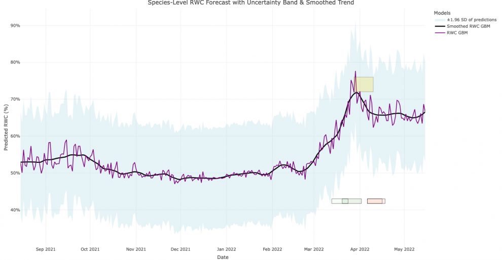 Figure 2. Example of seasonal RWC trajectory for Yakima, Washington (2021–2022), generated using the gradient boosting machine (GBM) model.
Cold hardiness (LT, LT50 and LT10). The Cold Hardiness panel shows predicted lethal temperature thresholds (LT, LT10, LT50) with the option to overlay Tmin for frost risk interpretation (Figure 3).
When daily minimum atmospheric temperature (Tmin) data are available — uploaded by the user or retrieved from NASA POWER or Open-Meteo — the tool overlays Tmin on the cold hardiness panel. Shaded areas highlight periods in which Tmin drops below the predicted LT10 (orange) or LT50 (red) thresholds for frost risk interpretation. Line chart of predicted temperature in Fahrenheit (y-axis) versus date (x-axis).
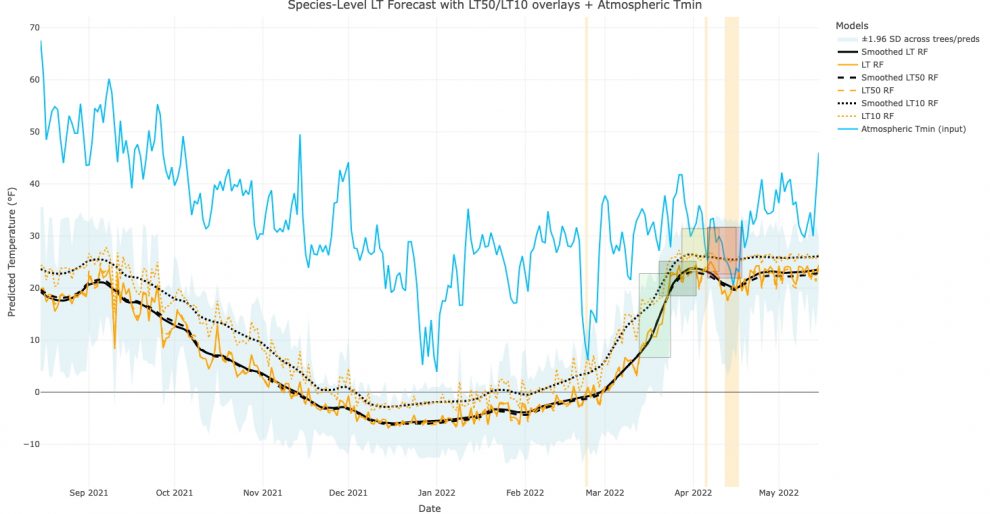 Figure 3. Example of cold hardiness output with Tmin overlay (blue) for Yakima, Washington (2021–2022), generated using the random forest (RF) model.
Using the tool
Step 1. Select a data source. Users can upload local weather data [required columns: Date (YYYY-MM-DD), J_date, Temp (°F) and Solar (MJ/m²); the optional Temp_min (°F) column enables Tmin overlay and frost risk shading] or retrieve the data via NASA POWER or Open-Meteo.
NASA POWER forecasts are generated for a seasonal window from August 15 to May 15, with options for regional presets or custom latitude and longitude input.
Step 2. Select forecast settings. Users can choose species-level forecasts or cultivar-specific predictions. Within the interface, different types of statistical models are available, including GLM, RF, NN, SVM and GBM. Uncertainty bands are displayed around predictions, and interpretation guidance is provided in the application legend.
Step 3. Run the forecast and download outputs. After selecting data inputs and forecast settings, click “Run Forecast”. Outputs are displayed in three panels: Cold Hardiness Forecast, Dormancy Progression (LTER) and Relative Water Content (RWC). Forecast tables can be downloaded as CSV files for further analysis.
Line chart of predicted LTER (y-axis) versus date (x-axis).
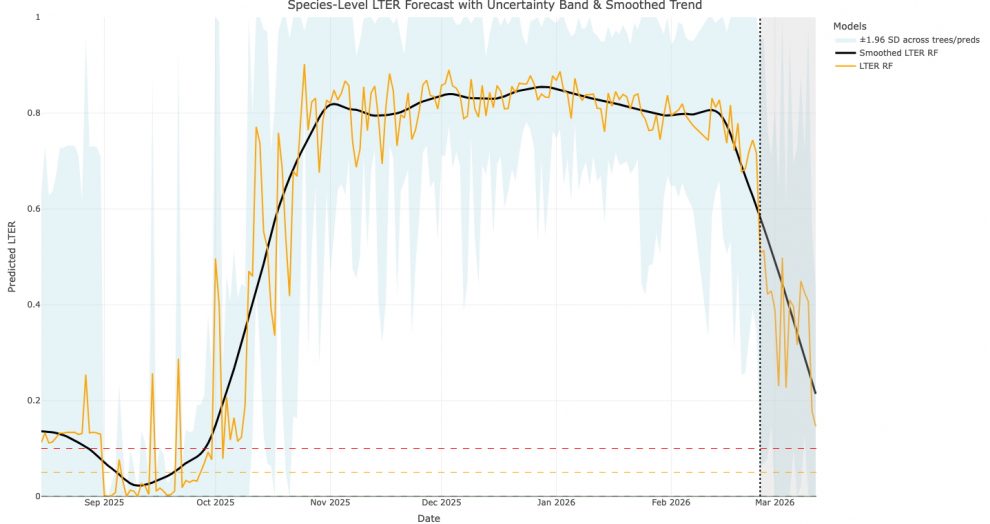 Figure 4. Example of LTER forecast for the 2025–2026 season in Prosser, Washington, generated using the random forest (RF) model. The grey area indicates the 14-day forecast window.
Disclaimer
This tool provides model-based seasonal estimates intended for decision support. Forecasts derive from historical relationships between climate and phenotype and may not capture extreme events, microclimatic variability or orchard-specific management effects.
NASA POWER data are gridded datasets representing area-average conditions that may differ from orchard-level measurements. Users should interpret results together with field observations and local experience.
The developer assumes no responsibility for crop damage or management outcomes resulting from the use of this tool. When available, data from local AgWeatherNet stations or orchard sensors are recommended.
Source: Fruit Matters, WSU
Opening image source: Stefano Lugli
Jonathan T. Magby
Yakima Valley College (formerly WSU-IAREC) - USA
Cherry Times - All rights reserved